I started posting Excel tips on my Linkedin page in early October 2020, and as of the 16th my "Did you know"post took the form it holds till this day. You can find my posts on Facebook, Instagram and Linkedin, all of which you can access via the links in the right hand column of this website.

October 26, 2020 - Did you know that Excel can tell you the date

October 23, 2020 - Did you know that Excel can tell you the date

October 22, 2020 - Did you know that Excel can tell you the date

October 21, 2020 - Did you know that Excel can tell you the date

October 20, 2020 - Did you know that Excel can tell you the date

October 16, 2020 - Did you know ..

I'm back with a little good to know "DID YOU KNOW" facts about excel. Today we're talking about Conditional Formatting. Did you know that there is a "Copy/Paste" function for conditional formatting. I love this

HOW TO:
First highlight the area where you just created a conditional format, click the "FORMAT" icon and then click and drag the range where you want to copy the formatting to.

201201

201202

201203

EXTENDED EXCELLENT EXCEL TIPS - December 2020

December 1, 2020 - Did you know .. Xmas Xcel edition ...

Now aside from being the color of a christmas tree (at least the logo is) there is actually so much more to Excel that is, or can be made to be, Christmasy. For the 1:st of December I thought we all use a little tool to help us get into, or stay in, a Christmas state of mind.

Here is an easy tutorial to creating your own Christmas tree, complete with presents and blinking lights.

Step 1:Highlight all the cells you need to create the GREEN part of the Christmas tree. Do this by holding CONTROL (PC) or COMMAND(mac)
Step2: Release the command/control button and enter "=RAND()". Finish by pressing command/control+ENTER. This enters the same formula in all highlighted cells.
Step 3: Center in the cells, then fill the cells with the green color of your choosing.
STEP 4:Go to CONDITIONAL FORMATTING and choose ICON sets.
Step 5: Edit the rule to be "show ICON only".
Step 6: Add a stump, and color it. Add presents, as many as you want. Change the width of all the columns to about 30 pixels. Add a seasons greetings ribbon somewhere.
Step 7: Press and hold F9 to make the lights blink.

December 2, 2020 - Did you know ...

Did you know that, as of today, there are 22 days left until Christmas. At least for those of us who celebrate on the 24th. Yesterday I showed you how to make a BLINKING CHRISTMAS TREE in EXCEL, and today I have made an ADVENT CALENDER to help keep you in that Christmas state of mind.

The basics of the tree and the boxes is all just filling cells, and the star is 3 INSERTED SHAPES (a star) in different sizes stacked on top of each other. I have made sure to MERGE the cells in each red box.

Then I entered this formula:
=IF(DATE(2020,12,2)=TODAY(),"THERE ARE 22 DAYS LEFT TILL CHRISTMAS","2")
In each red box, adjusting the DATE function and the TEXT so it is right for each day. What this formula does then is that when DATE function is equal to the TODAY function it will display text showing me how many days are left till Christmas, otherwise it will show me the date. You can adjust the text to whatever you want, and the size of the cells as well to make room for more text.

As a bonus I have added a MACRO that changes the size of the cell font so that the date can be displayed as a larger font.
ENJOY

December 3 2020 - Did you know ...

Did you know that THE TWELVE DAYS OF CHRISTMAS is a very long song? If you have ever heard it then you know it to be a very true story. And a hardship that comes with a very long song is remembering the lyrics.

The easiest way would of course be to just jot them down and look and them, but that would not be as much fun as making an EXCEL flash card game to learn the lyrics.

What I did what write each days lyrics into 12 separate boxes, then make a cell that would only let me enter a number from 1 to 12 and then some conditional formatting that would hide every other day than then one I wanted to look at. Nice and simple right.

If you have any questions regarding how the inner workings functions, as a question in the comments.

December 4, 2020 - Did you know ...

Sorry for the late posting today .. but then again it is Friday and I am allowed to be a bit lazy sometimes. Today's tip is more something for the years to come, as we already know what day of the week Christmas will fall on ... right.

Well, let's say that we don't know .. or that we are planning our Christmas for next year and we want to know what day of the week the 25th of December and the 1st of January falls on so we know which days we get off from work and how many vacation days we would need to add to make our vacation last as long as possible.

By using the date function:
=DATE(2020,12,25) or =DATE(2021,1,1)

You can substitute the date with a cell value if you have a column or row of years. But this will of course only display the date in the format of our choosing. This is where we get fancy. By CUSTOM FORMATTING the cells with "dddd" we get the formula to show us the day of the week.

December 5, 2020 - Did you know ...

Did you know that EXCEL could make even Santa's job easier. Let's take Santas list as an example. I have constructed a quick list that consists of a number of names and a few requirements to remain on the "NICE" list.

Step 1 is figuring out if the child in question has done all the things required on the NICE list. As it is important that they have a "YES" value in each cell, I have used an IF function with an AND function in it. This looks at every cell in the row and asks if has the value "YES". If it does then the child gets a gift, otherwise coal.

Step 2, conditional formatting to find the children who get coal.

Step 3, figuring out why the child gets goal. What I did here was use another IF function, with a text string for the "VALUE WHEN FALSE". For the VALUE WHEN TRUE I am using an INDEX, function with a nested MATCH function with a little concatenation sprinkled in for fun.

Check it out and see what you think.

December 6, 2020 - Did you know ...

Did you know that today is second advent. Now most people celebrate this by lighting the second of the four advent candles. Me being an EXCEL guy, I went another route. I have made my own advent candles in EXCEL.

The basic shape of the candles is made by simply filling cells with color. I shaped out the flames by holding down CONTROL and clicking on all the boxes that I wanted to be in my candle flame. When the last box is clicked enter the function:
=RAND() ... then press CONTROL+ENTER to enter the same formula in every chosen cell. Then I used CONDITIONAL FORMATTING and chose the ICON SET to add color to the changing values. I changed the GREEN color to YELLOW (could have been red, doesn't make any difference). Then I copy pasted a second candle with flame, and then copy pasted two more candles with no flame. The text inside the candles is for good measure. Once everything is in place, press and hold F9 to see your flames flicker.

Man EXCEL is really great.

December 7, 2020 - Did you know ...

So this week I thought I would start out with a formula that might not seem as useful on the surface, but once you get in and start getting creative with it .. it really turns into something great. The INDEX function. Basically the index function works like this:
=INDEX(array to search in, what row, what column) - return value

And you would think that you could then just let your cell be equal to that other cell and be done with it. But what if you need to look around in different cells but you want the value always returned in the same cell.

In my example I have a table of the 9 planets, their relative position, diameter and number of satellites. And I have set up two DATA VALIDATION LISTS to let me choose different variables. I am then using the INDEX function, with VLOOKUP to find my row number and HLOOKUP to find my column number. That formula looks like this:
=INDEX(B3:E11,VLOOKUP(G7,B3:F11,5,0),HLOOKUP(H7,C2:E12,11,0))

Just imagine the possibilities with this set up. Endless amounts of fun. As always, if you have any questions just comment below.

December 8, 2020 - Did you know ...

Did you know that there is this amazing thing called FLASH FILL. It is a part of the sort AI aspect of EXCEL and it can do some seriously amazing things to help you out.

In today's example I have acquired a list of 100 random emails that I would like to group by their providers. So what I need is a way to extract the provider from each email address and put that into its own column so that I can then order that in ascending order. What I don't want to do is sit and read of each address and type the provider name by hand. This is where FLASH FILL comes in handy.

With the list placed in column A, I type the provider name from the first two email addresses into column B. I am basically taking the text written between the "@" and the first "." With two solid examples of what I am doing I can simply mark the next PROVIDER cell and press CONTROL+E (same for both MAC and PC), and EXCEL will fill in my entire column for me. Easy peasy and I've got a list that I can now work with.

Dcember 9, 2020 - Did you know ...

Did you know that you can use the FIND and/or REPLACE function within EXCEL in order to adjust massive amounts of text. In our first table we have several issues that are affecting the user friendliness of the text inside it:
1: The > and < surrounding the country names
2: The hyphen in the middle of the person names
3: The text "at a private company" in the last column is unnecessary.

Begin by highlighting the area that you want to remove/replace. The > and < need to be removed in two steps, one symbol at a time. When removing the hyphen, you have to make sure that you add a SPACE (place cursor in the REPLACE WITH box and press the space bar once). For all steps enter the symbol or text string that you want to remove into the FIND WHAT box.

December 10, 2020 - Did you know ...

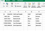
Today's #didyouknow will be in the spirit of what we learned yesterday. More text manipulation. It is not uncommon, when importing massive amounts of data into #EXCEL, that information gets lumped together into one column. So what do you do. Now you can use Tuesday's tip and set up for a flash fill, but there is another way that goes a bit faster in this case.

In picture one you can see a small sample set of ID, country, first and last name. After highlighting all the rows that we want to manipulate, we go to the #DATAtab and choose #texttocolumn; then using the #delimited setting we can press next; then we select that different delimiters that are separating our information; after making sure that preview is correct select finish and see the results. If you finish right away you will replace your old column with the newly divided information. But you can also go with next again and select another destination for your information.

December 11, 2020 - Did you know ... Did you know that you can use something called #hyperlink in #excel to allow you to quickly navigate between different tabs in a large document. It is pretty cool if you ask me.

In my example I have set up a small table with with 3 cells that I want to couple together with their respective tabs. What you have to imagine here is that the front/start tab consists of hundreds-thousands of cells and that the information in the tabs is just far too big to have on the start tab.

Simply right click on the first cell that you wish to assign a #hyperlink to and choose hyperlink from the bottom of the menu. Select the option "this document" and then select the tab from the menu. Once you are done your text will alter color and become underlined, signifying that you have hyperlinked it. Repeat for the other cells.

Come back tomorrow and I will show you how to create the "BACK" button that allows you navigate as easily to the start tab. If you have a question, comment below.

December 12, 2020 - Did you know ...

Did you know that yesterday I left you all with a bit of cliffhanger ... Maybe that is an overly dramatic way of putting it, but I did promise to tell you how to create a button that you can #hyperlink.

Basically, this works more or less the same as it does when hyperlinking a cell. There is a bit of work that needs to be done first though. In the #insert tab, choose #shapes and there pick the shape you want. Move your cursor down to the document and click and drag to place the shape (also choosing what size you want, this can always be altered later). Then right click on the shape and edit text to put a text on the button. Once you've done right click on the shape again and choose hyperlink; then, select where you want it to link to. Once you've done that the button is an active hyperlink, so if you want to edit it in anyway you have to right click it.

Look over the pictures posted to see the steps in real life. If you have any questions, comment below. Come back to tomorrow for the third advent.

December 13, 2020 - Did you know ...

I bet a lot of you actually #didknow that today is the third advent. That means today we light the third of our four advent candles. In honor of that I am bringing back my little lovely #exceladvent candles.

From last week, when only two candles were lit I have simply copy and pasted the candle light from candle 2 to candle 3. All the formatting comes along with it, so I did not need to add anything to it. The formula in each cell is simply =RAND(). Then, once you're done with all that and everything looks nice .. just press and hold F9 and your candle flames will flicker for you.

Enjoy the holidays.

December 14, 2020 - Did you know ...

Today we are going into the future .. so to speak. I will show you how EXCEL can help you #predict/ #forecast the future.

There is a lovely #function called #forecast.linear that will look at the numbers that you have in a sequence and predict the coming number/numbers. In my example I have a table the is showing me the amber of customers, sales and returns that I have had for a number of years, and I want to see what I can expect to happen in the upcoming 3 years (assuming that my company continues to grow at the same rate)

Here is the formula:

=FORECAST.LINEAR($D21,$E16:$E20,$D$16:$D$20) for #of customers in 2020.

December 15, 2020 - Did you know ...

Did you know that you can make an #excel document that links directly to webpages or email addresses. Some of you are reading this and going .. Marcus, of course we do. But then I add to this, did you also know that you don't have to have the link look like an email address or a webpage. Did I get your attention there.

In today's example, I am showing you a made up example of a company staff list with their email addresses. Along with a direct link to the company website. Then I could include this in a send out to potential customers and they would have a click-a-ble link to me.

Today we begin with linking the company name to the company website. We start by right clicking on the cell with the company name and choosing hyperlink. Then, on the website/file tab of hyperlinking I enter the website in the address slot. Making sure to enter in the text I want to display in the "text to display" slot. Then you can click on the cell and it takes you to my website.

December 16, 2020 - Did you know ...

Did you know that there is even more things that you can do with #hyperlinks in #excel. Yesterday I showed you how to take a cell and make it link to a homepage, taking a cell with only text and making that text a hyperlink.

Well, when you enter an email address, Excel will always make that a hyperlink and sometimes you don't want that. So in today's example I will show you the simple way we remove a hyperlink. First step; I am highlighting all the cells that I don't want to hyperlink, right clicking and choosing "remove hyperlink". Easy as all that.

Come back tomorrow for more hyperlink-madness.

December 16, 2020 - Did you know ...

Did you know that I was not yet done geeking out over #hyperlink on #excel. Well, if you didn't know before .. I assume that this comment certainly tells the whole story. So far I have shown you how to take text in a cell and turn it into a hyperlink to a website, how to remove the hyperlink from email addresses and I have also previously shown how to use the hyperlink function to allow you to travel from tab to tab within an excel #workbook.

Today I will show you how to edit the TEXT TO DISPLAY and what a SCREEN TIP is. Getting access to both of these is done by right clicking on the cell/hyperlink and choosing EDIT LINK.

The SCREEN TIP is a small message that will appear when you hover the mouse cursor over the hyperlink. In this case I have made mine read "send me a question".

As for TEXT TO DISPLAY, I made mine say "send Marcus an email". This is a very aesthetic choice as I just find that this looks nicer than just having my email address showing.

December 18, 2020 - Did you know ...

Now I'm sure that there are many of you out there that already know that there are plenty of great things you can do to spice up a party by using #excel. Things like #bingo. Well, maybe not a party .. but who doesn't love BINGO.

In the coming days I will show you how to build an excel document that you can use for any type of bingo you like. Fill it in with your own facts/things, make the board as big as you want it to be or spice up the appearance however you like.

Today we will look at making your sheet. You will want two tabs:
1. One for the #bingoboard, with as many copies as you like.
2. One for the list of items you want in the sheet.

It is rather smart (necessary) to make the cells on sheet two(where you write your facts) and the cells in the #bingosheets (so that you can set fonts and sizes from the get go).

You can see in my pictures how a plain and simple bingo sheet can look. Keep all your facts in a single column. And make sure you turn off AUTOMATIC FORMULA CALCULATION. You can turn it back on for other sheets, but for this one it needs to be set to manual. I will explain why later.

December 19, 2020 - Did you know ...

Did you know that last night I left you with a blank #bingosheet. Today I will address that and give you the #formula to fill in the sheet with.

One change from yesterday. I said that it was important to keep all the facts in one column, that turned out not to be necessary. Have as many columns there as you like .. so I've added a second to illustrate that.

Now, to fix the #bingoboard .. we begin by highlighting all the cells in the board, then going to the formula field and enter this:
=IFERROR(INDEX('Fact sheet'!$A:$B, RANDBETWEEN(2,51),RANDBETWEEN(1,2)),"")

Press Command+Enter(MAC) or Ctrl+Enter for PC.

#iferror is there in case something does not work and will return blank cell. Then we are using #index, which returns the value in the row number and column number indicated. For that we are using #randbetween. In the formula it returns a row from 2-51 and a column from 1-2 (A-B). After that you can copy the entire board and paste it into the other boards.

Come back tomorrow to find out why some squares are red.

December 20, 2020 - Did you know ...

Well, here we are on the #fourthadvent. This is the last one before #christmas. I know you were all expecting the continuation of my #bingo thread, but that will continue tomorrow. As for today.

Reopen your #adventcandle file, which you have of course all made and saved since the first advent, and lets make some adjustments. Copy the flame from the third candle and paste it on top of candle number four. Then, something that I should have done from the beginning as well, adjust the heights of the candles so it looks as if they have been used. Then just press and hold F9 and enjoy the your advent candles, brought to you by #excel, #randbetween and some basic cell filling and fun.

December 21, 2020 - Did you know ...

Did you know that we are returning back to #bingo now. Today I will explain to you how #excel helps me make sure that I don't have any duplicates on any given sheet.

If you remember the pictures from Saturday, there were some cells that were red with red text. So what I did was add a bit of #conditionalformatting to warn me about duplicates by coloring those cells. Using "format only unique or duplicate values" and choose #duplicatevalues.

Now, to get a sheet with no duplicates, go to the #formulatab and click on #calculatenow as many times as needed until your sheet is devoid of duplicates. Here is also the reason that formula calculation is set to manual, because otherwise every change you make to the sheet will recalculate the cells. Which could be annoying if you've finally got a sheet with no red cells.

Come back tomorrow for another step forward in #bingo evolution.

December 22, 2020 - Did you know ...

Did you know that I have yet another level to #excel #bingo. So there is this great version of bingo called #minglebingo. At least that is how I know it. It is a great way to help/force people at a party to mingle. Basically, before the event, everyone sends you 1 or 2 (or more) strange/funny facts about themselves. Now, you can put that into the #bingosheet that I have already shown you. But you need to make sure that they get everything right.

For this I created an answer board that looks at the fact on the board, and then using a double/nested #vlookup function to get the name of the person who submitted the fact. Here is that #formula:
=IFERROR(VLOOKUP(B3,'Fact sheet'!$A$2:$D$166,4,0),VLOOKUP(B3&"",'Fact sheet'!$A$2:$D$166,5,0))

You can see on the fact sheet that I have 1 column for facts, 1 for first name, 1 for last name and lastly 1 column where the first and last names are combined so the full name shows up in the answer sheet. I did this cause I wanted to alphabetize by their first names.

Remember that #calculationoptions must be set to #manual. This is to ensure that the board you print out and the answer sheet are a match.

December 23, 2020 - Did you know ...

Today, or rather tonight, being the day before Christmas for those of us living in Sweden. I only have one tip. Have an EXCELlent evening and enjoy the holidays

201204

201205

201206

201207

201208

201209

201210

201211

201212

201213

201214

201215

201216

201217

201218

201219

201220

201221

201222

201223